Concept Overview
A system of linear equations is a set of two or more linear equations with the same variables. Solving the system means finding the values that make all equations true at the same time. This often represents finding where two lines intersect, either in the coordinate plane or in real-world contexts like comparing costs or rates.
Key Vocabulary
- System of Equations: A set of equations with the same variables.
- Solution: A value or set of values that satisfies all equations in the system.
- Consistent System: A system with at least one solution.
- Inconsistent System: A system with no solution.
- Dependent System: A system with infinitely many solutions (the equations represent the same line).
Solving Systems by Graphing
The graphing method involves drawing each linear equation on the same coordinate plane. The solution to the system is the point where the two lines intersect — this point satisfies both equations. This method helps visualize the relationship between equations and identify whether a system has one solution, no solution, or infinitely many.
Example: Solve by Graphing
Solve the system:
\( y = 2x + 1 \)
\( y = -x + 4 \)
Step 1: Plot both lines using slope-intercept form \( y = mx + b \).
- The first line has slope 2 and y-intercept 1.
- The second line has slope -1 and y-intercept 4.
Step 2: Identify the point of intersection. The lines cross at \( (1, 3) \).
Solution: \( x = 1, y = 3 \) → The solution is \( (1, 3) \).
Solving Systems by Substitution
The substitution method works by solving one of the equations for a variable, and then substituting that expression into the other equation. This reduces the system to a single equation with one variable, which can then be solved algebraically.
Example: Solve by Substitution
Solve the system:
\( \textcolor{#005f99}{y = 3x – 2} \)
\( \textcolor{#cc5500}{x + y = 10} \)
Step 1: One equation is already solved for \( y \), so we substitute.
Step 2: Substitute \( \textcolor{#005f99}{y = 3x – 2} \) into the second equation:
\[ \begin{aligned} &\textcolor{#cc5500}{x + y = 10} \\ &\Rightarrow \textcolor{#cc5500}{x} + \textcolor{#005f99}{(3x – 2)} = \textcolor{#cc5500}{10} \\ &\Rightarrow 4x – 2 = 10 \Rightarrow 4x = 12 \Rightarrow x = 3 \end{aligned} \]
Step 3: Substitute \( x = 3 \) into the first equation to solve for \( y \):
\[ \begin{aligned} &y = 3(3) – 2 = 9 – 2 = 7 \end{aligned} \]
Solution: \( (3, 7) \)
Solving Systems by Elimination
The elimination method works by combining two equations to eliminate one of the variables. This is typically done by adding or subtracting the equations. It is most effective when both equations are in standard form:
Standard Form of a Linear Equation
\( Ax + By = C \)
If one variable has equal and opposite coefficients, you can eliminate it directly. Otherwise, multiply one or both equations to create a match—this process is called scaling the system.
Example 1: Direct Elimination
Solve the system:
\( \textcolor{#005f99}{3x + 2y = 12} \)
\( \textcolor{#cc5500}{3x – y = 3} \)
Step 1: Subtract the second equation from the first:
\[ \begin{aligned} &\textcolor{#005f99}{(3x + 2y)} – \textcolor{#cc5500}{(3x – y)} = \textcolor{#005f99}{12} – \textcolor{#cc5500}{3} \\ &\Rightarrow 3y = 9 \Rightarrow y = 3 \end{aligned} \]
Step 2: Substitute \( y = 3 \) into one of the original equations:
\( 3x + 2(3) = 12 \Rightarrow 3x + 6 = 12 \Rightarrow x = 2 \)
Solution: \( (2, 3) \)
Example 2: Multiply to Eliminate
Solve the system:
\( \textcolor{#005f99}{2x + 3y = 7} \)
\( \textcolor{#cc5500}{5x – 2y = 4} \)
Step 1: Eliminate one variable by scaling:
- \( \textcolor{#005f99}{2x + 3y = 7} \times 2 \Rightarrow \textcolor{#005f99}{4x + 6y = 14} \)
- \( \textcolor{#cc5500}{5x – 2y = 4} \times 3 \Rightarrow \textcolor{#cc5500}{15x – 6y = 12} \)
Step 2: Add the new equations:
\[ \begin{aligned} &\textcolor{#005f99}{4x + 6y} + \textcolor{#cc5500}{15x – 6y} = \textcolor{#005f99}{14} + \textcolor{#cc5500}{12} \\ &\Rightarrow 19x = 26 \Rightarrow x = \frac{26}{19} \end{aligned} \]
Step 3: Substitute back to solve for \( y \):
\[ \begin{aligned} &2\left(\frac{26}{19}\right) + 3y = 7 \Rightarrow \frac{52}{19} + 3y = 7 \\ &\Rightarrow 3y = 7 – \frac{52}{19} = \frac{81}{19} \Rightarrow y = \frac{27}{19} \end{aligned} \]
Solution: \( \left(\frac{26}{19}, \frac{27}{19} \right) \)
Note: It’s completely valid for systems to have fractional solutions—this just means the lines intersect at a non-integer point.
Interpreting Solutions to a System
A system of linear equations can have one solution, no solution, or infinitely many solutions. Each case corresponds to a different relationship between the lines on a graph.
One Solution (Intersecting Lines)
When two lines intersect at exactly one point, the system has one solution. This point satisfies both equations.
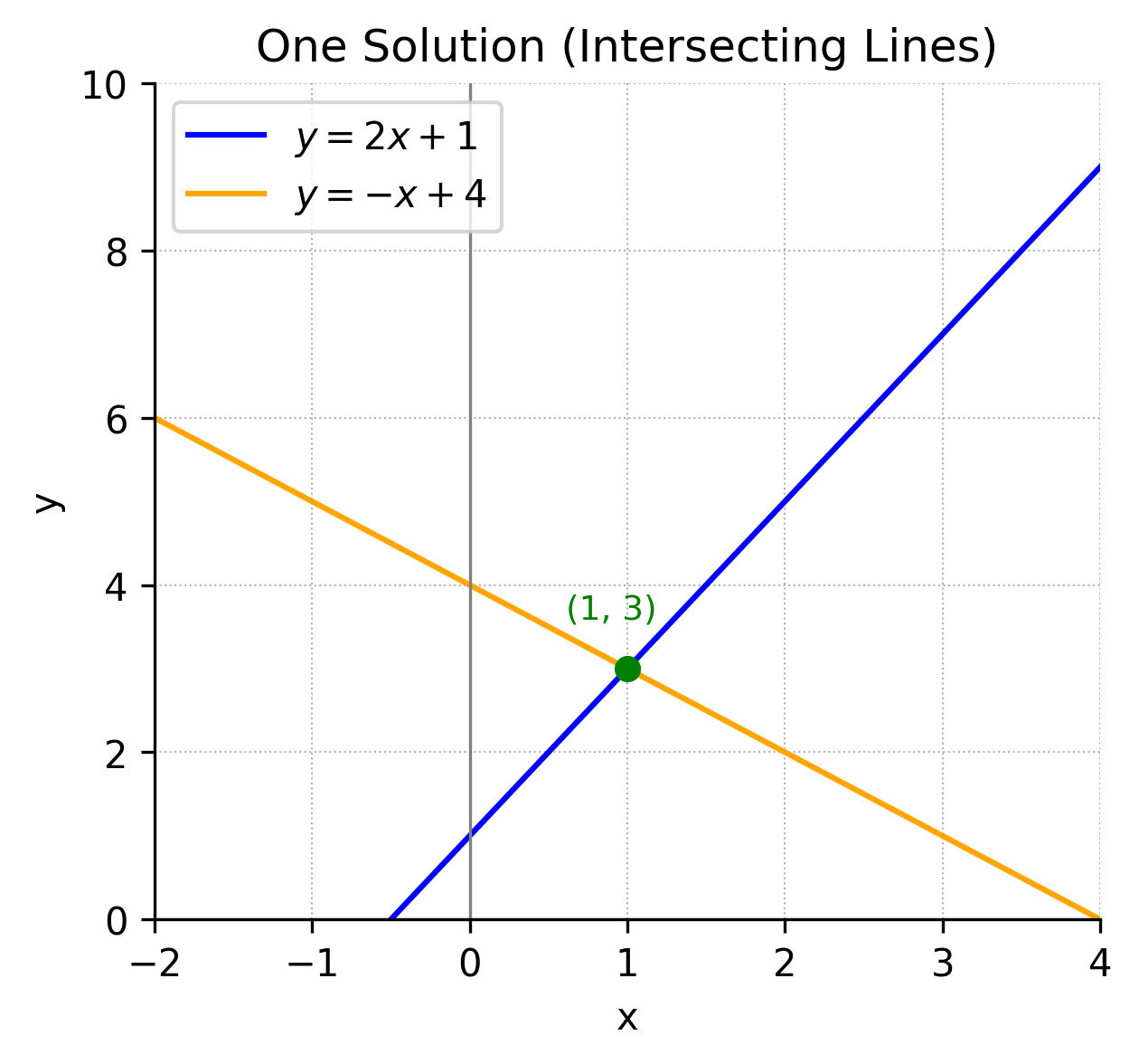
Example:
\( y = 2x + 1 \)
\( y = -x + 4 \)
Solution: \( (1, 3) \)
No Solution (Parallel Lines)
When the lines are parallel and never intersect, there is no solution. These lines have the same slope but different y-intercepts.
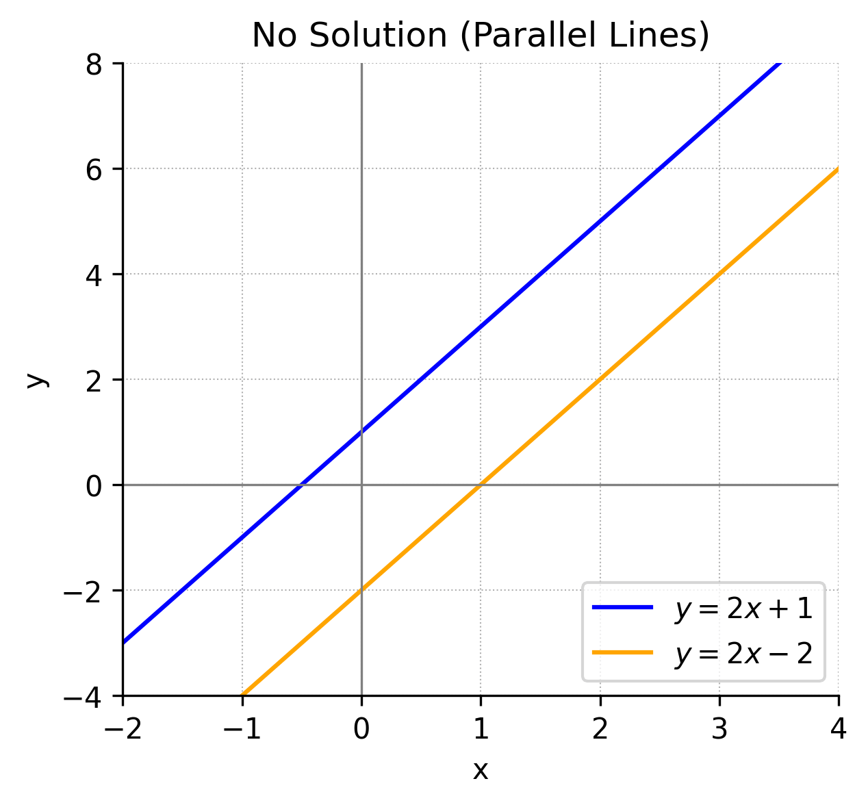
Example:
\( y = 2x + 1 \)
\( y = 2x – 2 \)
No solution.
Infinite Solutions (Same Line)
If the two equations describe the same line, then every point on that line is a solution to the system.

Example:
\( y = 2x + 1 \)
\( 4x – 2y = -2 \)
Same line → infinitely many solutions.
Try It Yourself!
- Solve by graphing:
\( y = \frac{1}{2}x + 1 \),
\( y = -x + 4 \) - Solve the system by substitution:
\( y = x + 4 \),
\( 2x + y = 1 \) - Solve by elimination:
\( 4x + 2y = 14 \),
\( -4x + y = -4 \)
Reveal Answers
- Graph both lines. They intersect at \( (2, 2) \)
- Substitute into second equation: \( 2x + (x + 4) = 1 \Rightarrow 3x = -3 \Rightarrow x = -1 \), then \( y = -1 + 4 = 3 \) → \( (-1, 3) \)
- Add equations: \[ \begin{aligned} &4x + 2y = 14 \\ &-4x + y = -4 \\ \hline &(4x + 2y) + (-4x + y) = 14 + (-4) \\ &0x + 3y = 10 \\ &3y = 10 \Rightarrow y = \frac{10}{3} \end{aligned} \] then back-substitute into \( -4x + y = -4 \) to find: \( -4x + \frac{10}{3} = -4 \Rightarrow -4x = -\frac{22}{3} \Rightarrow x = \frac{11}{6} \)
Connections & Extensions
Systems of equations appear in real-life applications such as budgeting, comparing phone plans, or solving mixtures. In computer science and engineering, systems help model constraints. Later, systems of equations extend into matrix algebra and are used to solve multi-variable problems efficiently.